One issue I had with the previous machine learning model I built was the inability to add more than one sound directly after each other. I had to wait about 1 second before starting the next sound for the machine learning model to recognise it  (I know it doesn’t sound like much, but trust me – IT IS!)

That’s frustrating and not acceptable. Let’s fix this! 💪🏽

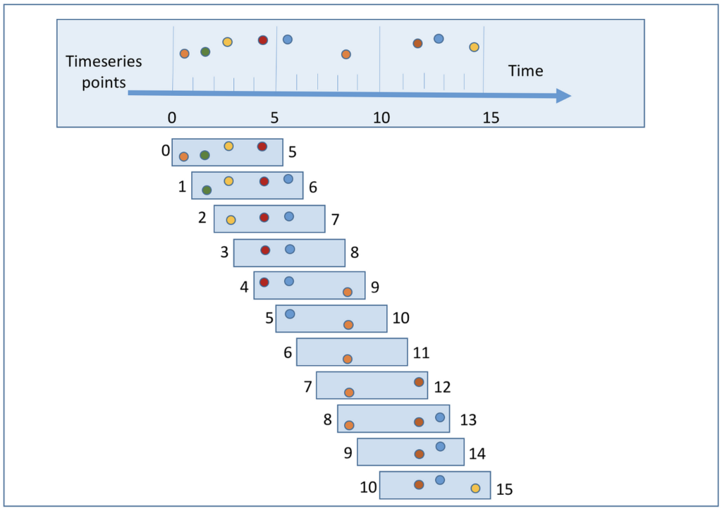
After extensive research, we identified that time series data is crucial for our needs. It can significantly improve our model’s performance. 🏎️

So, what did we do?

1. Made the Window Size Smaller 🤏🏽

• We adjusted the window size to be shorter. Why? Because the samples are brief, and we want it to be just long enough to capture the longest possible sound, which is “takatak” at 750 milliseconds.

2. Decreased the “Window Increase” Interval 🪟

• We reduced the window increase interval to 100ms. Why? Because if the model only updates every half a second, it can only predict at those intervals. By making the window increase more gradual, the model can catch sounds more accurately and promptly.

3. Actual BIG BOSS: Spectral Analysis 👸🏽

• Spectral analysis is awesome, she is the real game-changer here! Last time, we talked about using Mel-Frequency Cepstral Coefficients (MFCC), which are super cool. This time, we are also adding spectral analysis alongside MFCC. This extra step allows the model to examine the waveform itself to detect a “doom” or a “tak” based on its shape. More on Spectral Analysis in the next blog!